A complete reproducible analysis
analysis.RmdThis vignette walks one end-to-end analysis: snapshot the database, build a provenance-stamped dataset, profile it, and export — everything documented so the result can be reproduced later.
1. Snapshot, then connect
The database may be live under EntropIA. Before analysis, take a
snapshot with entropia_copy() and run against
that, so the analysis is immune to writes landing mid-run and
the provenance records a stable source.
con <- entropia_connect(system.file("extdata", "entropia-example.sqlite", package = "entropiaR"))
snap <- tempfile(fileext = ".sqlite")
entropia_copy(con, snap)
snap_con <- entropia_connect(snap)
entropia_disconnect(con) # original connection no longer needed
2. Build the analysis dataset
entropia_analysis_dataset() applies filters to the
corpus, collects it, and stamps provenance. This is the boundary:
everything after it is ordinary tibble work, and everything before it is
recorded.
corpus <- entropia_analysis_dataset(snap_con, name = "corpus_full")
corpus
#> entropia_dataset: corpus_full
#>   schema: 0029_rag_chunks  content: 09d4c603b66d
#> # A tibble: 5 × 19
#>   item_id      item_title collection_id metadata item_created_at item_updated_at
#>   <chr>        <chr>      <chr>         <chr>            <int64>         <int64>
#> 1 22222222-22… Manifiest… 11111111-111… "{\"__e…   1768478460000   1768478520000
#> 2 22222222-22… Manifiest… 11111111-111… "{\"__e…   1768478460000   1768478520000
#> 3 22222222-22… Manifiest… 11111111-111… "{\"__e…   1768478460000   1768478520000
#> 4 22222222-22… Fotografí… 11111111-111…  NA        1768478700000   1768478760000
#> 5 22222222-22… Carta al … 11111111-111… "{\"__e…   1768478580000   1768478640000
#> # ℹ 13 more variables: collection_name <chr>, collection_description <chr>,
#> #   collection_created_at <int64>, collection_updated_at <int64>,
#> #   asset_id <chr>, asset_path <chr>, asset_type <chr>, asset_size <int>,
#> #   asset_created_at <int64>, asset_sort_index <int>, parent_asset_id <chr>,
#> #   page_number <int>, text <chr>
entropia_provenance(corpus)
#> entropiaR dataset provenance
#>   name:           corpus_full
#>   schema version: 0029_rag_chunks
#>   content hash:   09d4c603b66d68c4c0cef0f51ff09a04fb30a49fe200907ef69693d11dd25732
#>   source path:    /tmp/RtmpG2NdhL/file1edd58424b23.sqlite
#>   package:        0.0.0.9000
#>   built at:       2026-08-24T01:10:27.977Z
#>   R version:      R version 4.6.1 (2026-06-24)
3. Temporal profile
When were assets created? entropia_temporal_profile()
buckets a date column. Collect the asset accessor directly —
entropia_collect() types its millisecond timestamps to
POSIXct, which the profiler requires:
assets <- entropia_assets(snap_con) |> entropia_collect()
temporal <- entropia_temporal_profile(assets, created_at, unit = "second")
temporal
#> # A tibble: 5 × 2
#>   created_at              n
#>   <dttm>              <int>
#> 1 2026-01-15 12:07:00     1
#> 2 2026-01-15 12:07:10     1
#> 3 2026-01-15 12:07:20     1
#> 4 2026-01-15 12:07:30     1
#> 5 2026-01-15 12:07:40     1
4. Document lengths
entropia_document_lengths() appends character and word
counts per document to any tibble carrying a text column:
texts <- entropia_text(snap_con) |> entropia_collect()
lengths <- entropia_document_lengths(texts)
lengths |> select(id, n_chars, n_words)
#> # A tibble: 5 × 3
#>   id                                   n_chars n_words
#>   <chr>                                  <int>   <int>
#> 1 33333333-3333-4333-8333-333333333331      50       9
#> 2 33333333-3333-4333-8333-333333333332      54       7
#> 3 33333333-3333-4333-8333-333333333333      NA      NA
#> 4 33333333-3333-4333-8333-333333333334      NA      NA
#> 5 33333333-3333-4333-8333-333333333335      23       4
Empty text counts as 0; NA text stays
NA.
5. Entities
entropia_entities() excludes soft-deleted rows by
default and surfaces provenance (source model) per entity.
entropia_entity_frequency() tallies them by type:
entities <- entropia_entities(snap_con) |> entropia_collect()
entropia_entity_frequency(entities)
#> # A tibble: 3 × 3
#>   entity_type  value                     n
#>   <chr>        <chr>                 <int>
#> 1 organization Sindicato Ferroviario     1
#> 2 person       Juan Pérez                1
#> 3 place        Plaza de Mayo             1
6. Topics
Topics are normalized UPPERCASE names. Join item_topics
to topics, then tally:
item_topics <- entropia_item_topics(snap_con) |> entropia_collect()
topics <- entropia_topics(snap_con) |> entropia_collect()
entropia_topic_frequency(left_join(item_topics, topics, by = c("topic_id" = "id")))
#> # A tibble: 2 × 2
#>   name          n
#>   <chr>     <int>
#> 1 HUELGA        1
#> 2 SINDICATO     1
7. Collections side by side
entropia_compare_collections() summarizes the corpus per
collection:
entropia_compare_collections(corpus)
#> # A tibble: 1 × 4
#>   collection_name   n_items n_assets     n
#>   <chr>               <int>    <int> <int>
#> 1 Archivo de prueba       3        5     5
8. Corpus quality
entropia_corpus_quality() reports OCR coverage,
transcription presence, and empty texts per asset type, plus metadata
coverage per collection:
quality <- entropia_corpus_quality(snap_con)
quality
#> # A tibble: 10 × 5
#>    metric                 group                 n total    pct
#>    <chr>                  <chr>             <int> <int>  <dbl>
#>  1 empty_text             audio                 0     1  0
#>  2 empty_text             image                 0     0 NA
#>  3 empty_text             pdf                   0     2  0
#>  4 metadata_coverage      Archivo de prueba     2     3  0.667
#>  5 ocr_coverage           audio                 0     1  0
#>  6 ocr_coverage           image                 0     1  0
#>  7 ocr_coverage           pdf                   2     3  0.667
#>  8 transcription_presence audio                 1     1  1
#>  9 transcription_presence image                 0     1  0
#> 10 transcription_presence pdf                   0     3  0
9. Visualize
entropia_plot_* helpers wrap the analysis summaries in
ggplot2 (Suggests) and return ordinary ggplot objects you
can extend:
entropia_plot_temporal(temporal)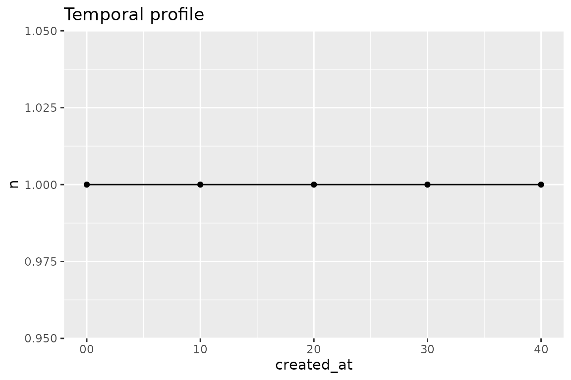
entropia_plot_entities(entropia_entity_frequency(entities))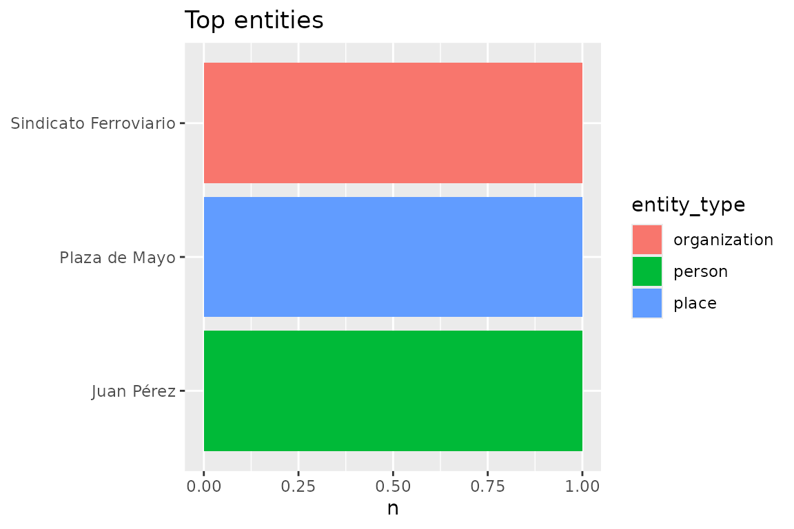
entropia_plot_coverage(quality)
#> Warning: Removed 1 row containing missing values or values outside the scale range
#> (`geom_col()`).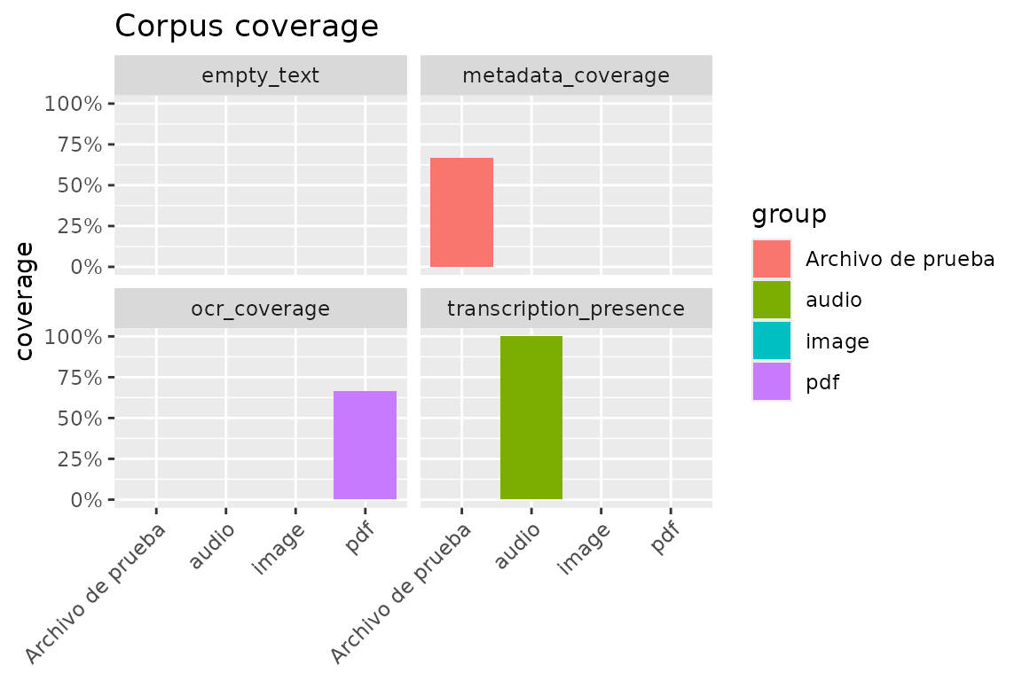
10. Export with provenance
The dataset exports as-is (RDS keeps its class and provenance; CSV is streamed for lazy inputs). Always write the provenance sidecar alongside:
export_path <- tempfile(fileext = ".csv")
entropia_export(entropia_corpus(snap_con), export_path)

rds_path <- tempfile(fileext = ".rds")
entropia_export(corpus, rds_path, format = "rds")
prov_path <- tempfile(fileext = "-prov.json")
entropia_write_provenance(corpus, prov_path)
The RDS round-trips with its provenance intact:
back <- readRDS(rds_path)
entropia_provenance(back)[["name"]]
#> [1] "corpus_full"
Cleanup
entropia_disconnect(snap_con)That is the loop: snapshot → build a stamped dataset → analyze → export with a sidecar. Each step uses functions documented elsewhere in this site; the provenance records the whole chain.